Optional Lab: Logistic Regression

In this ungraded lab, you will

• explore the sigmoid function (also known as the logistic function)
• explore logistic regression; which uses the sigmoid function

import numpy as np
%matplotlib widget
import matplotlib.pyplot as plt
from plt_one_addpt_onclick import plt_one_addpt_onclick
from lab_utils_common import draw_vthresh
plt.style.use('./deeplearning.mplstyle')

Sigmoid or Logistic Function

As discussed in the lecture videos, for a classification task, we can start by using our linear regression model, $f_{\mathbf{w},b}(\mathbf{x}^{(i)}) = \mathbf{w} \cdot \mathbf{x}^{(i)} + b$, to predict $y$ given $x$.

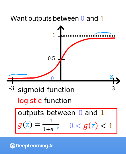
• However, we would like the predictions of our classification model to be between 0 and 1 since our output variable $y$ is either 0 or 1.
• This can be accomplished by using a "sigmoid function" which maps all input values to values between 0 and 1.

Let's implement the sigmoid function and see this for ourselves.

Formula for Sigmoid function

The formula for a sigmoid function is as follows -

$g(z) = \frac{1}{1+e^{-z}}\tag{1}$

In the case of logistic regression, z (the input to the sigmoid function), is the output of a linear regression model.

• In the case of a single example, $z$ is scalar.
• in the case of multiple examples, $z$ may be a vector consisting of $m$ values, one for each example.
• The implementation of the sigmoid function should cover both of these potential input formats. Let's implement this in Python.

NumPy has a function called exp(), which offers a convenient way to calculate the exponential ( $e^{z}$) of all elements in the input array (z).

It also works with a single number as an input, as shown below.

# Input is an array. 
input_array = np.array([1,2,3])
exp_array = np.exp(input_array)

print("Input to exp:", input_array)
print("Output of exp:", exp_array)

# Input is a single number
input_val = 1  
exp_val = np.exp(input_val)

print("Input to exp:", input_val)
print("Output of exp:", exp_val)

The sigmoid function is implemented in python as shown in the cell below.

def sigmoid(z):
    """
    Compute the sigmoid of z

    Args:
        z (ndarray): A scalar, numpy array of any size.

    Returns:
        g (ndarray): sigmoid(z), with the same shape as z
         
    """

    g = 1/(1+np.exp(-z))
   
    return g

Let's see what the output of this function is for various value of z

# Generate an array of evenly spaced values between -10 and 10
z_tmp = np.arange(-10,11)

# Use the function implemented above to get the sigmoid values
y = sigmoid(z_tmp)

# Code for pretty printing the two arrays next to each other
np.set_printoptions(precision=3) 
print("Input (z), Output (sigmoid(z))")
print(np.c_[z_tmp, y])

The values in the left column are z, and the values in the right column are sigmoid(z). As you can see, the input values to the sigmoid range from -10 to 10, and the output values range from 0 to 1.

Now, let's try to plot this function using the matplotlib library.

# Plot z vs sigmoid(z)
fig,ax = plt.subplots(1,1,figsize=(5,3))
ax.plot(z_tmp, y, c="b")

ax.set_title("Sigmoid function")
ax.set_ylabel('sigmoid(z)')
ax.set_xlabel('z')
draw_vthresh(ax,0)

As you can see, the sigmoid function approaches 0 as z goes to large negative values and approaches 1 as z goes to large positive values.

Logistic Regression

A logistic regression model applies the sigmoid to the familiar linear regression model as shown below:

$$ f_{\mathbf{w},b}(\mathbf{x}^{(i)}) = g(\mathbf{w} \cdot \mathbf{x}^{(i)} + b ) \tag{2} $$

where

$g(z) = \frac{1}{1+e^{-z}}\tag{3}$

Let's apply logistic regression to the categorical data example of tumor classification.
First, load the examples and initial values for the parameters.

x_train = np.array([0., 1, 2, 3, 4, 5])
y_train = np.array([0,  0, 0, 1, 1, 1])

w_in = np.zeros((1))
b_in = 0

Try the following steps:

• Click on 'Run Logistic Regression' to find the best logistic regression model for the given training data
  • Note the resulting model fits the data quite well.
  • Note, the orange line is '$z$' or $\mathbf{w} \cdot \mathbf{x}^{(i)} + b$ above. It does not match the line in a linear regression model. Further improve these results by applying a threshold.
• Tick the box on the 'Toggle 0.5 threshold' to show the predictions if a threshold is applied.
  • These predictions look good. The predictions match the data
  • Now, add further data points in the large tumor size range (near 10), and re-run logistic regression.
  • unlike the linear regression model, this model continues to make correct predictions

plt.close('all') 
addpt = plt_one_addpt_onclick( x_train,y_train, w_in, b_in, logistic=True)

Congratulations!

You have explored the use of the sigmoid function in logistic regression.